A query that ran in forty milliseconds last month now takes eleven seconds. Someone pastes a wall of indented text into the chat, with arrows, costs and words like "Hash Right Join", and the room goes quiet. EXPLAIN output looks like it was written for the database, not for you.
It was, in a sense. But it is also a very honest document, and a small amount of vocabulary lets you read most of it. This guide is for engineers who write SQL daily and have been nodding politely at query plans.
What a plan actually is
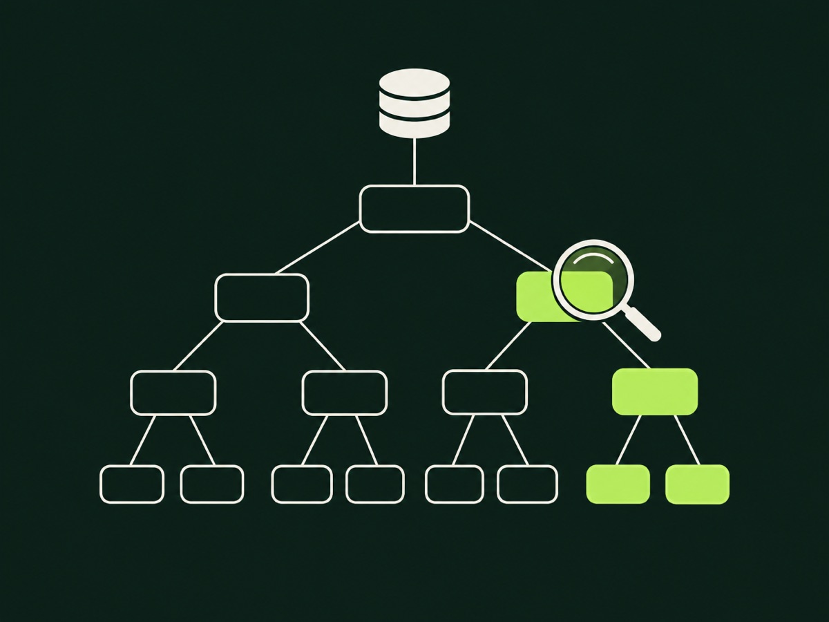
When you send a query, PostgreSQL does not run it as written. SQL says what you want. The planner decides how to get it: which indexes to use, in what order to join tables, and which join method to apply. The plan is that decision, shown as a tree.
Read it from the innermost, most indented lines outward. The deepest nodes run first and feed rows upward to their parents. The top line is the final result.
There are two commands to know. EXPLAIN shows the plan the planner would choose, with estimates, without running the query. EXPLAIN (ANALYZE, BUFFERS) actually runs the query and reports what really happened, including time and memory pages touched. Use the second for diagnosis. Be careful with it on statements that write data, because ANALYZE executes them. Wrap those in a transaction and roll back.
A first plan, line by line
Take a simple lookup:
EXPLAIN (ANALYZE, BUFFERS)
SELECT * FROM payments WHERE account_id = 4821;
A typical result looks like this:
Index Scan using payments_account_id_idx on payments
  (cost=0.43..52.10 rows=40 width=96)
  (actual time=0.031..0.210 rows=38 loops=1)
  Index Cond: (account_id = 4821)
  Buffers: shared hit=45
Planning Time: 0.120 ms
Execution Time: 0.260 ms
Break it down:
- Index Scan using ... is the method. The planner found an index on
account_idand used it. - cost=0.43..52.10 is the planner's own unit of effort, not milliseconds. The first number is the cost to return the first row, the second to return all rows. Compare costs within one plan, never across machines.
- rows=40 is the estimate. actual rows=38 is the truth. These are close, which is good.
- loops=1 says this node ran once. This number matters more than it looks, as we will see.
- Buffers: shared hit=45 means 45 pages were found in memory. A
readfigure would mean pages fetched from disk.
That is a healthy plan. Short, estimated well, and cheap.
Scan types you will meet
You will see the same handful of node types again and again.
Seq Scan reads the whole table. It is not automatically bad. For a small table, or a query that needs most rows, it is the fastest option. It is bad when it reads millions of rows to return a few.
Index Scan walks an index and fetches matching rows from the table. Index Only Scan answers entirely from the index when all needed columns are in it, skipping the table, provided the visibility information is up to date.
Bitmap Heap Scan sits between the two. It collects matching row locations from one or more indexes, then reads the table pages in order. You often see it when a filter matches a moderate share of rows, or when two indexes are combined.
The question is never "is there a Seq Scan". It is "does the amount of work match the number of rows I actually need".
Join methods
Joins have three main strategies, and each suits different shapes of data.
Nested Loop takes each row from the outer side and looks up matches on the inner side. It is excellent when the outer side is small and the inner side has an index. It is a disaster when the outer side is large and the inner lookup is slow, because the cost multiplies.
Hash Join builds an in memory hash table from one input and probes it with the other. It handles large, unsorted inputs well. If the hash table does not fit in work_mem, it spills to disk, and you will see batches greater than one.
Merge Join walks two sorted inputs together. It shines when both sides are already sorted, perhaps by index, and is common on big joins.
None is best. The planner picks based on estimated row counts, which brings us to the most important habit.
Compare estimates to actuals
Most slow plans have one cause: the planner guessed wrongly about how many rows it would see. It then picked a strategy that is right for the guess and wrong for reality.
Scan down the plan and compare rows= with the actual rows= for each node. A gap of a few percent is normal. A gap of ten times or a thousand times is the bug.
Nested Loop
  (cost=0.43..120.00 rows=5 width=64)
  (actual time=0.05..9800.00 rows=250000 loops=1)
Here the planner expected five rows and got a quarter of a million. It chose a nested loop for a few rows, then ground through a lot of them. The fix is not in the join, it is in the estimate.
Common reasons for bad estimates:
- Statistics are stale. Run
ANALYZEon the table, or check that autovacuum is keeping up. - Columns are correlated. The planner assumes
cityandpostcodeare independent, but they are not. Extended statistics withCREATE STATISTICScan describe the dependency. - A function or expression hides the column from statistics. A filter on
lower(email)has no stats unless there is an expression index. - The value is skewed. One tenant owns most rows, and the default sample does not capture it well. Raising the statistics target for that column can help.
The loops trap
The actual time on a node is the average per loop, not the total. A node showing actual time=0.5..0.6 with loops=40000 has really taken about twenty seconds in total. Multiply before you conclude.
This catches people constantly in nested loops. An inner index scan that looks instant becomes the whole cost because it ran forty thousand times. Look for large loops values on the inner side of a nested loop, and ask whether a hash join would suit better, or whether the outer side returned far more rows than expected.
Sorts, memory and disk
Look for Sort Method. quicksort Memory: 120kB is fine. external merge Disk: 340000kB means the sort spilled to disk because it exceeded work_mem. Before raising that setting globally, remember it applies per operation per connection, so a large value multiplied by many sessions can exhaust memory. Consider raising it for the specific session or query instead, or adding an index that delivers rows already sorted.
Similarly, a Rows Removed by Filter figure far larger than the rows returned is a sign that the database read lots of data and threw most of it away. An index on the filtered column, or a better composite index, usually helps.
Indexes that actually help
A few rules of thumb hold up well.
For a query that filters on equality and sorts or ranges on another column, put the equality column first in a composite index. For frequently filtered subsets, a partial index such as one covering only status = 'pending' can be much smaller and faster. For columns you only read, an INCLUDE clause can enable index only scans.
And be sceptical of adding indexes by reflex. Every index slows writes and takes space. Add one after reading a plan that proves it would change the access path, then confirm with a new plan.
A routine that works
When a query is slow, follow the same path every time. Run EXPLAIN (ANALYZE, BUFFERS) on realistic data, not an empty development database. Find the node with the largest actual time, remembering to multiply by loops. Compare estimated and actual rows around it. Decide whether the cause is statistics, a missing index, or the shape of the query. Change one thing, then run the plan again.
Plans stop being frightening once you notice they are just a list of steps with a guess and a result beside each. Keep a few past plans from your own system and read them when nothing is wrong. The day something is, you will already know what normal looks like.